
Analyzing commodity trading advisor’s is never an easy task. In analyzing a specific CTA manager for the first time, there are many different tools or statistical values that should be considered in order to determine whether or not a CTA’s strategy is investable. One of the most important areas of discussion during the initial due diligence process is the CTA’s ability to manage risk. In times of negative performance, how quickly does the manager cut its loss and realize they are wrong. What type of volatility should the investor expect? There are a handful of different statistical values that help assess risk, however in this article we will closely look at standard deviation and downside deviation and its importance when analyzing a CTA.
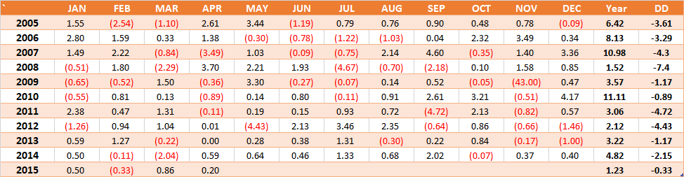
Most investors are familiar with standard deviation and how it can be used to measure risk. In its simplest terms, standard deviation is a measure of how spread out values are in a series of numbers/returns. In calculating the standard deviation, it gives investors a “standard” way of knowing what is normal, and what is outside the range of normality. A lower standard deviation is better, and it means returns are more likely to be in a narrower range, whereas a larger standard deviation means returns are more likely to be scattered. Let’s take the following monthly return stream and analyze how standard deviation will give us an idea of what to expect from the following CTA. See monthly return stream below beginning in January of 2005:
There is a substantial risk of loss in trading commodity futures, options and off-exchange foreign currency products. Past performance is not indicative of future results.
The monthly standard deviation for the above return stream is 1.60, with average monthly rate of return of 0.45% since January 2005. Having these two numbers allows us to set a “normal” range of expected monthly returns moving forward. The range can be calculated by adding and subtracting 1.60 (our monthly standard deviation) by our average monthly rate of return of 0.45%, which gives us a range of -1.15% to +2.05% . This means that it would be “normal” for future monthly returns to fall within that range.
Many investors use standard deviation to measure expected risk or volatility of a CTA, however is it the best measure of risk? Does it paint a clear picture of what we should expect on the downside? The answer is yes and no, depending on your analysis. Standard deviation takes into consideration downside volatility across a set of monthly returns, but it also takes into account upside volatility. However, should we be as concerned with the upside volatility (i.e. how scattered the positive months are)? Sure, it’s great to know the expected volatility for a specific strategy which includes both the upside and downside (exactly what the standard deviation give us), however if we only want to focus in on the downside volatility, a better risk measure to use is downside deviation.
Downside deviation only focuses on the volatility of negative returns (assuming MAR is set to 0). Downside deviation seeks to remedy the equal weighting of upside and downside volatility calculated in standard deviation by ignoring all of the “good” volatility and instead focusing on the “bad” returns. Similar to standard deviation, a lower downside deviation number is better. Since downside deviation might be a new term to many people, we will walk you through the calculation and how you come to this number.
Downside Deviation Calculation (5 Step Process):
Using the same monthly return stream as above, we follow the below steps in order to calculate downside deviation.
1) Define the minimum acceptable monthly return (MAR) you expect for a specific CTA investment. This is a number that you as the investor will decide and set. Since we would like to analyze all the negative returns, we will set the MAR to 0.
2) Subtract the MAR (which we set at 0) from the return for each period/month in the return stream.
3) After subtracting the MAR from each month’s return, if the return remains positive after subtracting the MAR then reset that value to 0. For example, April 2005 monthly return was 2.61. We proceed to subtract the MAR (in our case 0) and if the number remains positive we set that number to 0.
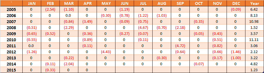
4) Square the differences and add all the numbers together.

5) Divide by the total number of months and take the square root. Finally take the square root of this number. This is the downside deviation.
- Sum of all the numbers together equals, 113.5293. 113.5293 divided by 124 (total number of months), equals 0.915559. Square root of 0.915559, equals 0.956848. The downside deviation for this monthly return stream is 0.96. The number of 0.96 shows us that with a MAR of 0, it is “normal” to have losing months that are within 0.96%. Negative returns outside or greater than 0.96% are considered “not normal”.
In the example in this article, the downside deviation of 0.96 is lower than the standard deviation of 1.60. This is good, because essentially it means that the downside volatility in this return stream is lower than the overall volatility (the combined volatility of negative AND positive months). If the reverse was true (where the downside deviation was higher than the standard deviation), that would mean that the CTA’s negative months are much more volatile than the CTA’s positive months. Both standard deviation and downside deviation have unique qualities in assessing risk and can be used differently to analyze a CTA strategy. We recommend using both statistics in comparison to one another in your analysis.