As we have previously discussed in our articles, there are many ways to analyze whether or not a commodity trading advisor (CTA) is worth investing with. From analyzing the underlying core of the strategy to various risk statistics, the list can go on and on. In past articles we have covered different types of risk statistics that help in our investment process, from Sharpe Ratio to Sortino ratio to downside deviation. Another value commonly reported on many of the CTA database’s is a term called skewness. What is skewness and how does it help assess the underlying CTA strategy?
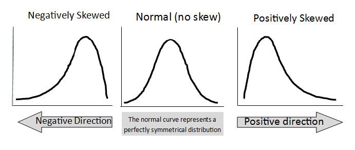
Skewness is measured as a coefficient, with the ability for the coefficient to be a positive, negative or zero. The coefficient of skewness is a measure for the degree of symmetry in the monthly return distribution. It allows investors the ability to determine where the majority of monthly returns are going to fall and also point out any outlier events. Let’s take a look at how skewness is measured and how it’s represented graphically:
|
Negatively skewed distribution |
Normal distribution |
Positively skewed distribution |
As we can see from the above images, if the left tail (tail at small end of the distribution) is more pronounced than the right tail (tail at the large end of the distribution), the function is said to have negative skewness. If the reverse is true, it has positive skewness. If the two are equal, it has zero skewness or a symmetrical distribution. By analyzing the skewness of a CTA, it allows us to determine where future returns could fall (past performance is not indicative of future results) and where the returns of “black swan” events could potentially fall. An understanding of the skewness of the dataset indicates whether potential deviations from the mean are going to be positive or negative.
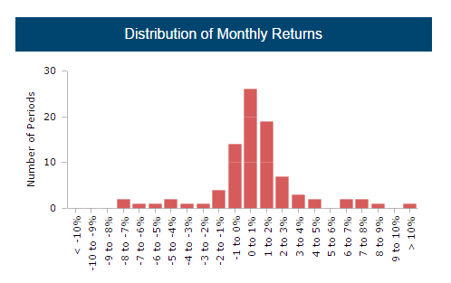
Let’s take the above information and see how it relates to a few different CTA’s strategies, and how it helps in our decision making process. Let’s take CTA Y’s monthly track record and monthly return distribution:
CTA Y

The skewness coefficient for CTA Y is 0.29. As you can see from the above information across 89 monthly data points, CTA Y has a slightly positive skew which means that the right tail is more pronounced than the left tail, with the right tail being longer. With the understanding of skewness from the above, we can make the generalization that any deviations from the mean are going to be slightly positive. This distribution of returns are asymmetrical, with a positive skew.
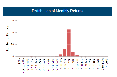
CTA Z

The skewness coefficient for CTA Z is -4.48. As you can see from the above information across 71 data points, CTA Z has a negative skew which means that the left tail is more pronounced than the right tail, with the left tail being longer. Although the returns for CTA Z seems to be more consistent and steady month to month, left tail events are more likely based on the skew.
All Skew is not created equal
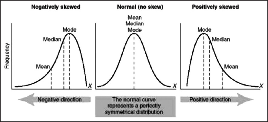
Unfortunately, looking at the skewness coefficient alone doesn’t paint the clearest of pictures. When analyzing the skewness coefficient across a set of data points, it is important to also measure it against the mean of the data points. By having a positive skew alone doesn’t justify that future returns will be positive, but rather means that the bulk of returns will lie to the left of the mean with extreme values to the right of the mean. Refer to the illustration below for further clarification:
- Skewness > 0 – Right skewed distribution – most values are concentrated on left of the mean, with extreme values to the right.
- Skewness < 0 – Left skewed distribution – most values are concentrated on the right of the mean, with extreme values to the left.
- Skewness = 0 – mean = median, the distribution is symmetrical around the mean.
A positive skew could be good or bad, depending on the mean. A positive mean with a positive skew is good, while a negative mean with a positive skew is not good. If a data set has a positive skew, but the mean of the returns is negative, it means that overall performance is negative, but the outlier months are positive. A negative skew is generally not good, because it highlights the risk of left tail events or what are sometimes referred to as “black swan events.” While a consistent and steady track record with a positive mean would be a great thing, if the track record has a negative skew then you should proceed with caution.
In conclusion, the skewness coefficient of a set of data points helps us determine the overall shape of the distribution curve, whether it’s positive or negative. The coefficient number also helps us determine whether the right tail or the left tail of the distribution is more pronounced. You cannot assess a CTA solely based on its skewness, however, in conjunction with other statistics and variables it allows us to have a more in-depth understanding of the consistency of returns and the potential left tail events in the future (past performance is not indicative of future results).


